Orthogonal AMP
Approximate message passing (AMP) [DMM09] is a signal recovery algorithm for models involving large random matrices. An attractive feature of AMP is that its dynamical behavior could be characterized precisely via a simple iteration called state evolution (SE), in the high dimensional limit. However, the SE technique of AMP only works for matrices with i.i.d. Gaussian distributed elements. Orthogonal AMP generalizes AMP in the sense that it admits state-evolution characterization for a larger class of random matrices.
Introduction
To gain some intuition about the SE of OAMP, let us consider the following recursion
\[ \begin{align} \mathbf{z}_{\mathsf{out}}^{t+1}= f_t\bigg( \mathbf{U}^T \, g_t(\mathbf{U}\mathbf{z}_{\mathsf{out}}^t) \bigg), \end{align} \]
where \(\mathbf{U}\) is a uniformly random (i.e., Haar-distributed) orthogonal matrix, and \(f_t,g_t:\mathbb{R}\mapsto\mathbb{R}\) satisfy the divergence-free condition [MP17]:
\[ \mathsf{div}_t(f):=\frac{1}{n}\sum_{i=1}^n f’([\mathbf{U}^T \, g(\mathbf{Uz}_{\mathsf{out}}^t) ]_i)=0.\quad\text{and}\quad \mathsf{div}_t(g):=\frac{1}{n}\sum_{i=1}^n g’([\mathbf{Uz}_{\mathsf{out}}^t]_i)=0. \]
In the above equations, the scalar functions \(f_t,g_t\) are applied to the input vectors in a component-wise fashion, namely, \([f(\mathbf{x})]_i=f(x_i)\). Given any function \(\hat{f}\), we could apply a divergence removal step and construct the following function
\[ f_t(\mathbf{x})=C_f\cdot\left( \hat{f}(\mathbf{x})- \left(\frac{1}{n}\sum_{i=1}^n \hat{f}(x_i)\right)\cdot \mathbf{x} \right), \]
where \(C_f\) is a constant. This function is divergence-free if the divergence term converges to a constant (in some probabilistic sense) as \(n\) tends to infinity. In what follows, we shall supress the time indices for \(f_t\) and \(g_t\), but we should keep in mind that these functions are not required to be the same at different iterations.
State evolution
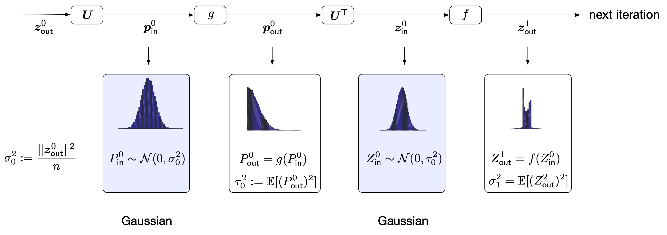
The iterative process can be represented by the following flow diagram
 |
Our goal is to understand the evolution of the empirical distributions of the vectors \(\{\mathbf{z}_{\mathsf{in}}^t,\mathbf{z}_{\mathsf{out}}^t,\mathbf{p}_{\mathsf{in}}^t,\mathbf{p}_{\mathsf{out}}^t\}\). (We may think of the empirical distribution of a vector as its histogram.) Suppose that the above recursion is initialized with a deterministic vector \(\mathbf{z}_{\mathsf{out}}^0\) satisfying \(\|\mathbf{z}_{\mathsf{out}}^0\|=\sigma_0\cdot \sqrt{n}\). Since \(\mathbf{U}\) is a Haar matrix, we have
\[ \mathbf{p}_{\mathsf{in}}^0=\mathbf{Uz}_{\mathsf{out}}^0\sim \|\mathbf{z}_{\mathsf{out}}^0\|\cdot \text{Unif}(\mathbb{S}^{n-1}), \]
where \(\text{Unif}(\mathbb{S}^{n-1})\) denotes a uniform distribution over the unit sphere. By the well-known connection between a uniform distribution over the sphere and an i.i.d. Gaussian distribution, we have
\[ \mathbf{p}_{\mathsf{in}}^0=\mathbf{Uz}_{\mathsf{out}}^0 \overset{dist}{=} \|\mathbf{z}_{\mathsf{out}}^0\|\cdot\frac{\mathbf{w}}{\|\mathbf{w}\|}=\frac{\sigma_0\sqrt{n}}{\|\mathbf{w}\|}\cdot \mathbf{w},\quad \mathbf{w}\sim\mathcal{N}(\mathbf{0},\mathbf{I}), \]
where \(\overset{dist}{=}\) denotes equivalence in distribution. As \(\|\mathbf{w}\|/\sqrt{n}\to 1\) almost surely by the law of large numbers, we expect
\[ \mathbf{p}_{\mathsf{in}}^0 \overset{iid}{\approx} {P}_{\mathsf{in}}^0\sim \mathcal{N}(0,\sigma_0^2). \]
Here, we introduced a shorthand \(\mathbf{x}\overset{iid}{\approx} X\) to denote that the empirical distribution of \(\mathbf{x}\) converges to that of the random variable \(X\). Similar arguments yield
\[ \begin{align} \mathbf{p}^0_{\mathsf{out}}:={g}(\mathbf{p}_{\mathsf{in}}^0) & \overset{iid}{\approx} {g}\left( P_{\mathsf{in}}^0\right), \nonumber\\ \mathbf{z}_{\mathsf{in}}^0:=\mathbf{U}^T\mathbf{p}^0_{\mathsf{out}} &\overset{iid}{\approx} Z_{\mathsf{in}}^0\sim\mathcal{N}(0,\tau_0^2)\quad \tau_0^2:=\mathbb{E}[(P^0_{\mathsf{out}})^2],\\ \mathbf{z}^{1}_{\mathsf{out}}:=f(\mathbf{z}^0_{\mathsf{in}}) &\overset{iid}{\approx} Z^1_{\mathsf{out}}={f}\left( Z^0_{\mathsf{in}}\right)\nonumber. \end{align} \]
See the following figure for illustration. The basic intuition behind the above results is that the vectors after the orthogonal transforms (either \(\mathbf{U}\) or \(\mathbf{U}^T\)) are Gaussian distributed, and the vectors after the nonlinear transforms are simply functions of the input Gaussian vectors. Furthermore, the variances of these Gaussian vectors could be calculated via a simple recursive formula which is often called state evolution [DMM09]. In this post, we will also use the term “state evolution” to refer to the overall process of characterizing the empirical distributions.
 |
If this kind of heuristic is correct, we could track the evolution of the distributions of \(\{\mathbf{z}_{\mathsf{in}}^t,\mathbf{z}_{\mathsf{out}}^t,\mathbf{p}_{\mathsf{in}}^t,\mathbf{p}_{\mathsf{out}}^t\}\) pretty easily. Unfortunately, the above heuristics can be problematic: note that \(\mathbf{p}_{\mathsf{out}}^0\) in Eq. (2) is generally correlated with \(\mathbf{U}\) (since it is a function of \(\mathbf{U}\)) and we do not know a priori whether such correlation would destroy the Gaussianality of \(\mathbf{U}^T\mathbf{p}_{\mathsf{out}}^0\). To elaborate on this point, consider an extreme case where \(\mathbf{p}_{\mathsf{out}}^0\) is aligned with the first column of \(\mathbf{U}\). In this case, \(\mathbf{U}^T\mathbf{p}_{\mathsf{out}}^0\propto \mathbf{e}_1\) and is certainly not close to an i.i.d. Gaussian random vector.
This is where the divergence-free properties of \(f\) and \(g\) come into play. Perhaps surprisingly, when \(f,g\) are divergence-free, \(g(\mathbf{p}_{\mathsf{in}}^t)\) and \(f(\mathbf{z}_{\mathsf{in}}^t)\) behave as if they are still ‘‘independent of’’ \(\mathbf{U}\) in each iteration, in the sense that heuristics such as Eq. (2) are still correct. A rigorous proof of this phenomenon has been carried out in [RSF19][Takeuchi20] using a conditioning method first developed in [Bolthausen14][BM11].
The following figure shows the numerical results of a simple experiment. In this experiment, we set \(\hat{f}(x)=5\tanh(x)\) and \(\hat{g}(x)=1.5|x|\). The functions \(f\) and \(g\) are the divergence-free versions of \(\hat{f}\) and \(\hat{g}\) (with \(C=1\)) respectively. We compared two schemes: one with \(\hat{f}\) and \(\hat{g}\) and the other with \(f\) and \(g\). We predicted the performances of both schemes using the state evolution procedure described in (2). The results in the figure shows a clear mismatch between the simulation results and the predictions for the naive scheme where \(\hat{f}\) and \(\hat{g}\) are used. In contrast, the predictions for the scheme with divergence-free functions are very accurate. Finally, we emphasize that, for computational complexity concerns, we did not use a actual Haar random matrix in this experiment but instead used \(\mathbf{U}=\mathbf{P}_1\mathbf{F}\mathbf{P}_2\), where \(\mathbf{P}_1\) and \(\mathbf{P}_2\) are two phase “randomization” matrices consisting of i.i.d. \(\pm1\) entries and \(\mathbf{F}\) is a \(5000\times5000\) discrete cosine transform (DCT) matrix. It is expected that the performance under a Haar random matrix is close to the structured one, as observed in [MP17].
 |
The transform \(\mathbf{U}^Tg(\mathbf{U}\mathbf{a})\)
Before we discuss the state evolution of (1), let's discuss some interesting properties of the transform \(\mathbf{U}^Tg(\mathbf{U}\mathbf{a})\). Suppose \(\mathbf{a}\) is a deterministic vector with \(\|\mathbf{a}\|=O(\sqrt{n})\). We argue that the transform \(\mathbf{U}^Tg(\mathbf{U}\mathbf{a})\) is equivalent to a linear function of \(\mathbf{a}\) plus an independent Gaussian term. More precisely, the following holds for large \(n\):
\[ \mathbf{U}^Tg(\mathbf{U}\mathbf{a})\approx \alpha \cdot \mathbf{a}+\text{Gaussian}, \]
where \(\alpha\) converges to a deterministic constant and Gaussian term has approximately i.i.d. zero-mean elements.
Special case
We first consider a special case: \(\mathbf{a}=\sqrt{n}\mathbf{e}_1\). In this case, we have \(\mathbf{Ua}=\sqrt{n}\mathbf{u}_1\) where \(\mathbf{u}_1\) is the first column of \(\mathbf{U}\). Denote \(\mathbf{U}=[\mathbf{u}_1,\mathbf{U}_{\backslash1}]\). We have
\[ \begin{align*} \mathbf{U}^Tg(\mathbf{Ua}) & = \begin{bmatrix} \mathbf{u}_1^T\\ \mathbf{U}_{\backslash1}^T \end{bmatrix} g(\mathbf{u}_1)\\ &= \begin{bmatrix} \mathbf{u}_1^T g(\mathbf{u}_1) \\ \mathbf{U}_{\backslash1}^T g(\sqrt{n}\mathbf{u}_1) \end{bmatrix}\\ &= \frac{\left(\mathbf{u}_1^T g(\sqrt{n}\mathbf{u}_1)\right)}{\sqrt{n}} \cdot \sqrt{n}\mathbf{e}_1 + \begin{bmatrix} 0 \\ \mathbf{U}_{\backslash1}^T g(\sqrt{n}\mathbf{u}_1) \end{bmatrix}. \end{align*} \]
Note that \(\mathbf{u}_1\sim \text{Unif}(\mathbb{S}^{n-1})\) and as discussed before
\[ \begin{align*} \frac{\mathbf{u}_1^T g(\sqrt{n}\mathbf{u}_1)}{\sqrt{n}} & = \frac{\sqrt{n}\mathbf{u}_1^Tg(\sqrt{n}\mathbf{u}_1)}{n}\\ &\to \mathbb{E}[Wg(W)]=\mathbb{E}[g’(W)]:=\alpha, \end{align*} \]
where \(W\sim\mathcal{N}(0,1)\) and the identity \(\mathbb{E}[Wg(W)]=\mathbb{E}[g’(W)]\) is known as Stein's lemma. For the second term, we note that for a Haar-distributed \(\mathbf{U}\), \(\mathbf{U}_{\backslash1}\) is uniformly distributed over the set of orthonormal matrices orthogonal to \(\mathbf{u}_1\). So, we could write \(\mathbf{U}_{\backslash1}\) as
\[ \mathbf{U}_{\backslash1} \overset{dist}{=} \mathbf{P}^{\perp}_{u_1} \widetilde{\mathbf{V}}, \]
where \(\mathbf{P}^{\perp}_{u_1}\in\mathbb{R}^{n\times {n-1}}\) is any basis matrix for the orthogonal space of \(\mathbf{u}_1\) and \(\widetilde{\mathbf{V}}\in\mathbb{R}^{(n-1)\times (n-1)}\) is a \((n-1)\)-dimensional Haar random matrix independent of \(\mathbf{u}_1\). In other words, \(\mathbf{P}^{\perp}_{u_1}\) summarizes the statistical correlation between \(\mathbf{U}_{\backslash1}\) on \(\mathbf{u}_1\) and \(\widetilde{\mathbf{V}}\in\mathbb{R}^{(n-1)\times (n-1)}\) reflects the remaining randomness. We can then study the distribution of the second term based on this representation:
\[ \begin{align*} \mathbf{U}_{\backslash1}^Tg(\sqrt{n}\mathbf{u}_1)&\overset{dist}{=}\widetilde{\mathbf{V}}^T\left( (\mathbf{P}_{u_1}^{\perp})^Tg(\sqrt{n}\mathbf{u}_1) \right)\\ &\overset{iid}{\approx} \frac{\|(\mathbf{P}_{u_1}^{\perp})^Tg(\sqrt{n}\mathbf{u}_1)\|}{\sqrt{n}}\cdot W\\ &=\sqrt{\frac{\|g(\sqrt{n}\mathbf{u}_1)\|^2 - \sqrt{n}\mathbf{u}_1^Tg(\sqrt{n}\mathbf{u}_1)}{n} }\cdot W\\ &\approx \underbrace{\sqrt{ \mathbb{E}[g^2(Z)] -\mathbb{E}^2[g’(Z)] }}_{\sigma_g} \cdot W, \end{align*} \]
where \(W\sim\mathcal{N}(0,1)\). Notice that the empirical distribution of \([0;\mathbf{U}_{\backslash1}^Tg(\sqrt{n}\mathbf{u}_1)]\) is the same as that of \(\mathbf{U}_{\backslash1}^Tg(\sqrt{n}\mathbf{u}_1)\) when \(n\to\infty\). Finally, we get the desired result
\[ \mathbf{U}^Tg(\mathbf{Ua})\overset{dist}{\approx} \alpha\cdot \mathbf{a}+\sigma_g \cdot \mathbf{w}. \]
with \(\mathbf{w}\sim\mathcal{N}(\mathbf{0},\mathbf{I})\).
General case
For simplicity, assume \(\|\mathbf{a}\|=\sqrt{n}\). Then, there exists a rotation matrix \(\mathbf{Q}\) such that
\[ \mathbf{a}=\mathbf{Q}(\sqrt{n}\mathbf{e}_1). \]
Hence,
\[ \begin{align*} \mathbf{U}^Tg(\mathbf{Ua}) &= \mathbf{U}^Tg(\mathbf{UQ}\sqrt{n}\mathbf{e}_1)\\ &=\mathbf{Q}\widetilde{\mathbf{U}}^Tg(\widetilde{\mathbf{U}}\sqrt{n}\mathbf{e}_1) \end{align*} \]
where \(\widetilde{\mathbf{U}}:=\mathbf{UQ}\) is still Haar distributed (and independent of \(\mathbf{Q}\)) by the rotational invariance of Haar measure. (Note \(\mathbf{Q}\) only depends on \(\mathbf{a}\) and is independent of \(\mathbf{U}\).) From the previous result, we have \(\alpha\cdot \sqrt{n}\mathbf{e}_1+\sigma_g \cdot [0;\mathbf{w}]\) and thus
\[ \begin{align*} \mathbf{U}^Tg(\mathbf{Ua}) &\overset{dist}{\approx} \mathbf{Q}\left(\alpha \sqrt{n}\mathbf{e}_1+\sigma_g \cdot \begin{bmatrix} 0\\ \mathbf{w} \end{bmatrix} \right)\\ &= \alpha\cdot\mathbf{a}+\sigma_g\mathbf{Q} \left( \begin{bmatrix} 0\\ \mathbf{w} \end{bmatrix} \right) \end{align*} \]
where the second term is again approximately i.i.d. Gaussian.
Why divergence-free
To see why \(f,g\) have to be divergence-free for approximations such as Eq. (1) to hold, let us consider \(\mathbf{z}_{\mathsf{in}}^{1}\):
\[ \mathbf{z}_{\mathsf{in}}^{1} =\mathbf{U}^T g\left(\, \mathbf{U} \mathbf{z}_{\mathsf{out}}^0\,\right). \]
Here, we emphasize that the initial vector \(\mathbf{z}_{\mathsf{out}}^0\) is independent of \(\mathbf{U}\). Since \(\mathbf{Uz}_{\mathsf{out}}^0\overset{iid}{\approx} P_{\mathsf{in}}^0\sim\mathcal{N}(0,\sigma_0^2)\), using the result in the previous section yields
\[ \begin{align*} \mathbf{z}_{\mathsf{in}}^{1} \approx\mathbb{E}[g’({P}_{\mathsf{in}}^0)]\cdot\mathbf{z}_{\mathsf{out}}^0+\text{Gaussian}. \end{align*} \]
Notice that \(\mathbf{z}_{\mathsf{out}}^0\) is initialized to be a fixed vector, and for subsequent iterations (namely, \(\mathbf{z}^t_{\mathsf{out}},t\ge1\)) it is the output of a non-linear function. In any case, the empirical law of \(\mathbf{z}^0\) (or \(\mathbf{z}^t_{\mathsf{out}},t\ge1\)) is generally non-Gaussian and we would want to remove its contribution in \(\mathbf{z}_{\mathsf{in}}^1\), i.e.,
\[ \mathbb{E}[g’({P}_{\mathsf{in}}^0)]=0, \]
which is nothing but the the divergence-free condition.
Alternatively, we can refer to the block diagrom shown in the first figure. If we want to establish orthogonality between \(\mathbf{z}_{\mathsf{in}}^{t+1}\) and \(\mathbf{z}_{\mathsf{out}}^{t}\) (output of \(f\) in the previous iteration), we should make the output of \(g\) to be orthogonal to its input, and this is guaranteed by the divergence-free property of \(g\). Due to the same reason, we see that \(f\) has to be divergence-free to ensure that \(\mathbf{p}^t_{\mathsf{in}}\) does not contain the contribution of \(\mathbf{p}^{t-1}_{\mathsf{out}}\), the non-Gaussian output of \(g\) from the previous iteration.
Until now, we only focused on the first iteration. More dedicated analysis is required to show that the non-Gaussian terms are correctly cancelled out for all subsequent iterations.
OAMP
OAMP is very close to (1) except that either \(f\) or \(g\) could also depend on the observations from which we wish to recover the signal. Suppose our observation is a component-wise nonlinear function of the signal \(\mathbf{x}_\star\), say, \(\mathbf{y}=\phi(\mathbf{Ux}_\star)\). Further, \(\mathbf{x}_\star\overset{iid}{=}X_\star\sim P_X\). (In the so-called phase retrieval problem, \(\phi(z)=|z|\).) Consider the following iteration where \(g\) is a function of both \(\mathbf{y}\) and \(\mathbf{U}\mathbf{z}_{\mathsf{out}}^{t}\):
\[ \mathbf{z}_{\mathsf{out}}^{t+1} = f\left( \mathbf{U}^T g(\mathbf{y},\mathbf{U}\mathbf{z}_{\mathsf{out}}^{t}) \right). \]
Since the nonlinearity \(\phi\) could be absorbed into \(g\), we will assume \(\mathbf{y}=\mathbf{Ux}_\star\) to simplify notation. The divergence-free condition on \(g\) now becomes
\[ \frac{1}{n}\sum_{i=1}^n\partial_2g( {y}_i,[\mathbf{U\mathbf{z}_{\mathsf{out}}^t}]_i )=0, \]
where \(\partial_2\) denotes partial derivative with respect to the second argument. We emphasize that \(g(\mathbf{y},\mathbf{Uz}^t_{\mathbf{out}})\) is no longer “independent of” \(\mathbf{U}\) is no longer correct. The reason is that \(g\) is not divergence-free with respect to the first argument. Nevertheless, the component of \(g\) that it orthogonal to \(\mathbf{Uz}_\star\) can still be treated as “independent of” \(\mathbf{U}\).
The state evolution should be slightly modified. We first decompose \(g\) as
\[ \begin{align*} g(\mathbf{Ux}_\star,\mathbf{Uz}_{\mathsf{out}}^t) &= \mathbb{E}[\partial_1 g]\cdot \mathbf{Ux}_\star + \mathbb{E}[\partial_2 g]\cdot \mathbf{Uz}_{\mathsf{out}}^t+\mathbf{w},\\ &= \mathbb{E}[\partial_1 g]\cdot \mathbf{Ux}_\star+\mathbf{w}, \end{align*} \]
where \(\mathbf{w}:=g-\mathbb{E}[\partial_1 g]\cdot \mathbf{Ux}_\star - \mathbb{E}[\partial_2 g]\cdot \mathbf{Uz}_{\mathsf{out}}^t\) is asymptotically orthogonal to both \(\mathbf{Ux}_\star\overset{iid}{\approx}\mathcal{N}\) and \(\mathbf{Uz}_{\mathsf{out}}^t\overset{iid}{\approx}\mathcal{N}\). The orthogonality can be verified based on the multivariate version of Stein's lemma:
\[ \mathbb{E}[Z_1 \eta (Z_2,Z_3)]=\mathbb{E}[Z_1Z_2]\mathbb{E}[\partial_1\eta(Z_2,Z_3)]+\mathbb{E}[Z_1Z_3]\mathbb{E}[\partial_2\eta(Z_2,Z_3)] \]
whenever \((Z_1,Z_2,Z_3)\) is jointly Gaussian. Using this representation of \(g(\mathbf{Ux}_\star,\mathbf{Uz}_{\mathsf{out}}^t)\), we obtain
\[ \begin{align*} \mathbf{U}^Tg(\mathbf{Ux}_\star,\mathbf{Uz}_{\mathbf{out}}^t) &= \mathbb{E}[\partial_1g]\cdot \mathbf{U}^T(\mathbf{Ux}_\star)+\mathbf{U}^T\mathbf{w}\\ &= \mathbb{E}[\partial_1g]\cdot\mathbf{x}_\star+\mathbf{U}^T\mathbf{w}, \end{align*} \]
where \(\mathbf{U}^T\mathbf{w}\) is (approximately) Gaussian and independent of \(\mathbf{x}_\star\) and \(\mathbf{z}_{\mathsf{out}}^t\). Compared with (1), the only difference is that the input to \(f\) is distributed as “signal plus independent Gaussian” instead of pure Gaussian. Also, to characterize \(g(\mathbf{Ux}_\star,\mathbf{Uz}_{\mathbf{out}}^t)\), we need to understand the joint distribution of \((\mathbf{Ux}_\star,\mathbf{Uz}_{\mathbf{out}}^t)\). Intuitively, both terms are zero-mean Gaussian, and we only need to specify their variances and covariance, both of which can be characterized via a recursive formula, similar to what we have shown before.